Online inverse linear optimization: Efficient logarithmic-regret algorithm, robustness to suboptimality, and lower bound
This post describes how to achieve the current best regret bound for online inverse linear optimization using the online Newton step (ONS), one of the main results in our recent paper. The method and analysis are very simple.
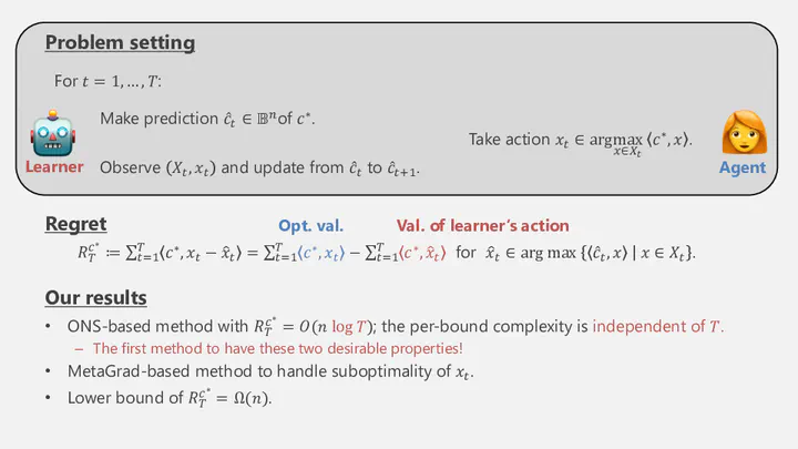
Problem Setting
Inverse optimization is the problem of estimating parameters of forward optimization problems based on observed optimal solutions. Let’s consider an agent who sequentially solves forward optimization of the following form $t = 1,\dots,T$:
$$ \mathrm{maximize}_{x \in \R^n} \quad {c^*}^\top x \qquad \mathrm{subject\ to} \quad x \in X_t, $$where $c^* \in \R^n$ is the agent’s internal objective vector, $X_t \subseteq \R^n$ is the $t$-th feasible set (which may be non-convex). Let $\mathbb{B}^n$ be the unit ball and assume the following conditions for simplicity:
- $X_1,\dots,X_t$ are contained in $\frac12\mathbb{B}^n$, and
- $c^*$ is also contained in $\frac12\mathbb{B}^n$.
For each $t$, let $x_t \in \mathop{\mathrm{\arg\,\max}}_{x \in X_t} {c^*}^\top x$ be an optimal solution taken by the agent.
The goal of inverse optimization is to estimate the agent’s objective vector $c^*$ based on the observed pairs of optimal solutions and feasible sets, $\{(x_t, X_t)\}_{t=1}^T$. Although this setting is elementary, it forms the basis for various problems of “inference from rational behavior,” such as inferring customers’ preferences from purchase history.
Online-Learning Approach
Bärmann, Pokutta, and Schneider (ICML 2017) presented an elegant online-learning approach to this problem. For each $t$, their method computes a prediction $\hat{c}_t$ of $c^*$ based on past observations, $\{(x_{i}, X_{i})\}_{i=1}^{t-1}$. Let $\hat x_t \in \mathop{\mathrm{\arg\,\max}}_{x \in X_t} {\hat c_t}^\top x$ denote the solution suggested by the prediction $\hat{c}_t$. A natural performance measure for those predictions is the regret:
$$ R_T^{c^*} \coloneqq \sum_{t=1}^T {c^*}^\top(x_t - \hat x_t), $$which represents the cumulative gap between the optimal values and objective values achieved by following the predictions $\hat{c}_t$. Bärmann et al. also defined another convenient measure that upper bounds the regret:
$$ \tilde R_T^{c^*} \coloneqq \sum_{t=1}^T (\hat c_t - c^*)^\top (\hat x_t - x_t) = \sum_{t=1}^T \hat c_t^\top (\hat x_t - x_t) + R_T^{c^*} \ge R_T^{c^*}, $$where the last inequality is due to $x_t, \hat x_t \in X_t$ and the optimality of $\hat x_t$ for $\hat c_t$. This measure suggests how online learning can be applied. Define $f_t\colon c\mapsto c^\top (\hat x_t - x_t)$ as the $t$-th cost function. Taking cost vectors, $\hat x_t - x_t$, to be chosen by an adversary, we can use standard online learning methods, such as the online gradient descent, to achieve
$$ R_T^{c^*} \le \tilde R_T^{c^*} = \sum_{t=1}^T (f_t(\hat c_t) - f_t(c^*)) = O(\sqrt{T}). $$This ensures that the average regret vanishes as $T \to \infty$. Let us refer to the formulation of Bärmann et al.—sequentially computing $\hat{c}_t$ to bound $R_T^{c^*}$—as online inverse linear optimization.
Logarithmic Regret via Ellipsoid-Based Method
In general online linear optimization (OLO), the regret bound $O(\sqrt{T})$ is tight. So, is $R_T^{c^*} = O(\sqrt{T})$ also tight for online inverse linear optimization? The answer is no:
- Besbes et al. (COLT 2021, Oper. Res. 2023) achieved $R_T^{c^*} = O(n^4 \log T)$, and
- Gollapudi et al. (NeurIPS 2021) achieved $R_T^{c^*} = O(n \log T)$,
where $n$ is the dimension of the space where $c^*$ lies.
Their idea is novel and somewhat different from the online-learning approach, which I briefly describe here. Intuitively, the feedback $(x_t, X_t)$ is informative compared to that in general OLO; the optimality of $x_t \in X_t$ narrows down the possible existence of $c^*$ to the normal cone of $X_t$ at $x_t$ (or loosely, the half-space normal to $x_t - \hat x_t$). Their methods implement this idea by sequentially updating a region that is ensured to contain $c^*$. Based on the volume argument commonly used in the analysis of the ellipsoid method, they established logarithmic regret bounds. However, the per-round time complexity is polynomial in $n$ and $T$, as their methods need to maintain the region specified by up to $T$ observations.
Our Approach: Online Newton Step
We provide a simple method such that:
- it achieves a regret bound of $R_T^{c^*} = O(n \log T)$ (matching the best known bound by Gollapudi et al.), and
- the per-round time complexity is polynomial in $n$ and independent of $T$.
Our approach is close to Bärmann et al., but we apply the online Newton step (ONS) to different cost functions $f_t$.
ONS is an online convex optimization (OCO) method that achieves the logarithmic regret for exp-concave losses. We say a twice differentiable function $f\colon \R^n \to \R$ is $\alpha$-exp-concave on $\mathcal{K} \subseteq \R^n$ if $\nabla^2 f(x) \succeq \alpha \nabla f(x) \nabla f(x)^\top$ for all $x \in \mathcal{K}$.
Regret bound of ONS (Hazan et al. 2007, Theorem 2).
Let $\mathcal{K}$ be a convex set with diameter $D$ and $f_1,\dots,f_T\colon\R^n\to\R$ be $\alpha$-exp-concave loss functions. Assume $\| \nabla f_t(x) \| \le G$ for all $t$ and $x \in \mathcal{K}$. Let $\hat c_1,\dots,\hat c_T \in \mathcal{K}$ be the outputs of ONS. Then, for any $c^* \in \mathcal{K}$, it holds that
$$\sum_{t=1}^T (f_t(\hat c_t) - f_t(c^*)) = O\left( n\left( \frac{1}{\alpha} + GD \right) \log T \right).$$Our method simply applies ONS to appropriate exp-concave functions $f_t$. Let $\eta = 1/2$ (the reason for this choice will be clear later) and define $f_t\colon \R^n \to \R$ by
$$ f_t(c) \coloneqq - \eta (\hat c_t - c)^\top (\hat x_t - x_t) + \eta^2 \left( (\hat c_t - c)^\top (\hat x_t - x_t) \right)^2, $$where $x_t$ is the agent’s optimal solution, $\hat c_t \in \frac12\mathbb{B}^n$ is the $t$-th prediction, and $\hat x_t \in \mathop{\mathrm{\arg\,\max}}_{x \in X_t} {\hat c_t}^\top x$.
Consider applying ONS to the above $f_t$, restricting the domain to $\frac12\mathbb{B}^n$.
To derive a regret bound, we need to evaluate the parameters, $G$, $D$, and $\alpha$, in the ONS regret bound.
In fact, these parameters are all constants.Here is the detailed calculation.
For simplicity, let $g_t = \hat x_t - x_t$, which satisfies $\| g_t \| \le 1$ since $\hat x_t, x_t \in X_t \subseteq \frac12\mathbb{B}^n$.
- Since the domain is $\frac12\mathbb{B}^n$, we have $D = 1$.
- By using $c, \hat c_t \in \frac12\mathbb{B}^n$, $\| g_t \| \le 1$, and $\eta = 1/2$, we have $$\| \nabla f_t(c) \| = \| \eta g_t - 2\eta^2 g_tg_t^\top (\hat c_t - c)\| \le \eta + 2\eta^2 \le 1$$ and $$\nabla f_t(c) \nabla f_t(c)^\top = \eta^2 \left( 1 - 2 \eta g_t^\top (\hat c_t - c) \right)^2 g_t g_t^\top \preceq \eta^2 (1 + 2\eta)^2 g_t g_t^\top = 2\nabla^2 f_t(c),$$ hence $G = 1$ and $\alpha = \frac{1}{2}$.
Thus, those parameters are constant for $\eta = 1/2$.
Therefore, ONS applied to $f_t$ satisfies
$$ \sum_{t=1}^T (f_t(\hat c_t) - f_t(c^*)) = O\left(n\log T \right). $$The remaining task is to bound $\tilde R_T^{c^*} = \sum_{t=1}^T (\hat c_t - c^*)^\top (\hat x_t - x_t)$, which upper bounds the regret $R_T^{c^*}$. For convenience, define
$$ V_T^{c^*} \coloneqq \sum_{t=1}^T \left( (\hat c_t - c^*)^\top (\hat x_t - x_t) \right)^2. $$Due to $\hat c_t, c^* \in \frac12\mathbb{B}^n$, $\hat x_t, x_t \in X_t \subseteq \frac12\mathbb{B}^n$, and $(\hat c_t - c^*)^\top (\hat x_t - x_t) \ge 0$ (by the optimality of $\hat x_t$ and $x_t$ for $\hat c_t$ and $c^*$, respectively), we have
$$ V_T^{c^*} \le \sum_{t=1}^T (\hat c_t - c^*)^\top (\hat x_t - x_t) = \tilde R_T^{c^*}. $$By using this and $f_t(\hat c_t) = 0$, which follows from the definition of $f_t$, we have
$$ \tilde R_T^{c^*} = - \sum_{t=1}^T \frac{f_t(c^*)}{\eta} + \eta V_T^{c^*} \le \sum_{t=1}^T \frac{f_t(\hat c_t) - f_t(c^*)}{\eta} + \eta \tilde R_T^{c^*}. $$With $\eta = 1/2$, we obtain
$$ \frac{\tilde R_T^{c^*}}{2} \le 2\sum_{t=1}^T (f_t(\hat c_t) - f_t(c^*)) = O(n\log T), $$thus establishing $R_T^{c^*} \le \tilde R_T^{c^*} = O(n\log T)$.
Related Topics
The above definition of $f_t$ and the proof strategy are inspired by those used in MetaGrad (Van Erven and Koolen NeurIPS 2016, Van Erven et al. JMLR 2021). Interestingly, using MetaGrad, instead of ONS, adds robustness against the suboptimality of the agent’s solutions, which is also discussed in our paper.
We have also obtained a regret lower bound of $R_T^{c^*} = \Omega(n)$. On the other hand, Gollapudi et al. showed a regret upper bound of $\exp(O(n \log n))$. Whether we can remove the dependence on $T$ while maintaining polynomial dependence on $n$ is an interesting open problem.
Another paper of ours in AISTATS 2025 also studies online inverse linear optimization. It views the problem as online convex optimization of a Fenchel–Young loss (Blondel et al. JMLR 2020) and presents a finite regret bound under the assumption that the agent’s forward problems have a gap between the optimal and suboptimal objective values.